
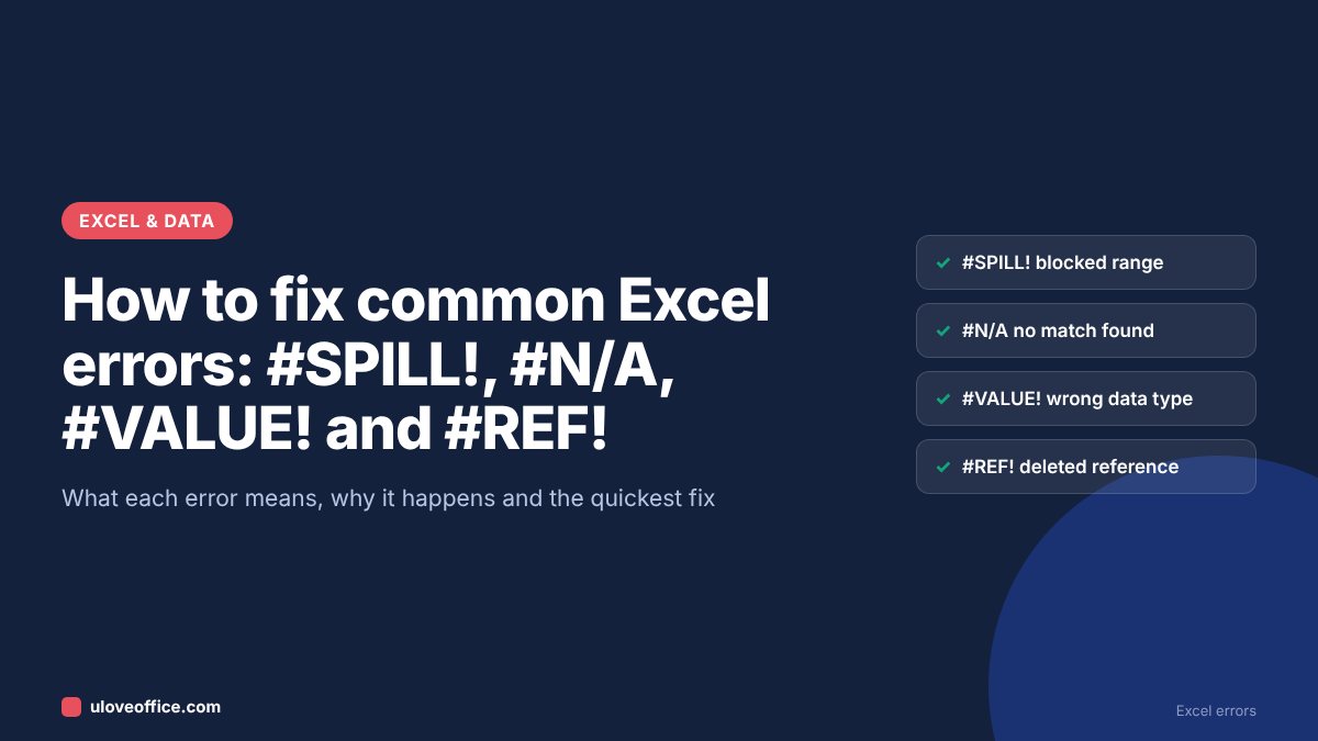
How to fix common Excel errors: #SPILL!, #N/A, #VALUE! and #REF!
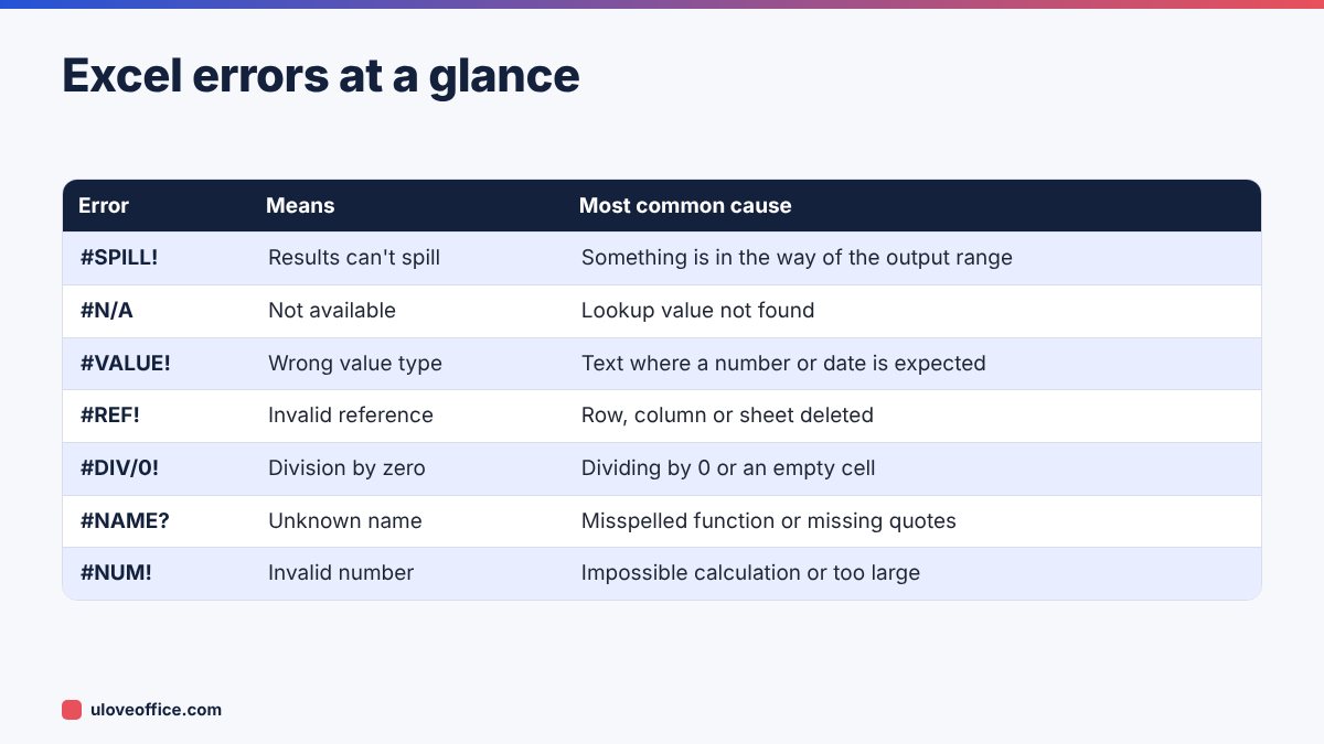
Quick answer: Each Excel error tells you what went wrong. #SPILL! means a dynamic array formula cannot output its results because cells in the way are not empty. #N/A means a lookup found no match. #VALUE! means a formula received the wrong type of data, often text instead of a number. #REF! means a formula refers to cells that were deleted. #DIV/0! means division by zero or a blank cell. #NAME? means Excel does not recognise a function or name, usually a typo. #NUM! means an impossible calculation. Click the error cell, use the small warning icon or Formulas > Evaluate Formula, find the cause and fix the data or formula, rather than hiding the error.
Errors are not failures; they are messages. Learning to read them turns a frustrating spreadsheet into a fixable one. This guide covers the errors office workers meet most often, with real causes and fixes.
Tools for finding the cause
Before fixing, find the exact cause:
- The warning icon: click the error cell, then the small yellow diamond for a short explanation and options such as “Show Calculation Steps”.
- Evaluate Formula: Formulas > Evaluate Formula steps through a formula one part at a time, showing where the error appears.
- Trace Precedents: Formulas > Trace Precedents draws arrows to the cells a formula uses. One of them may contain the error.
- F9 trick: in the formula bar, select part of a formula and press F9 to see its result. Press Esc afterwards so you do not overwrite the formula.
#SPILL!
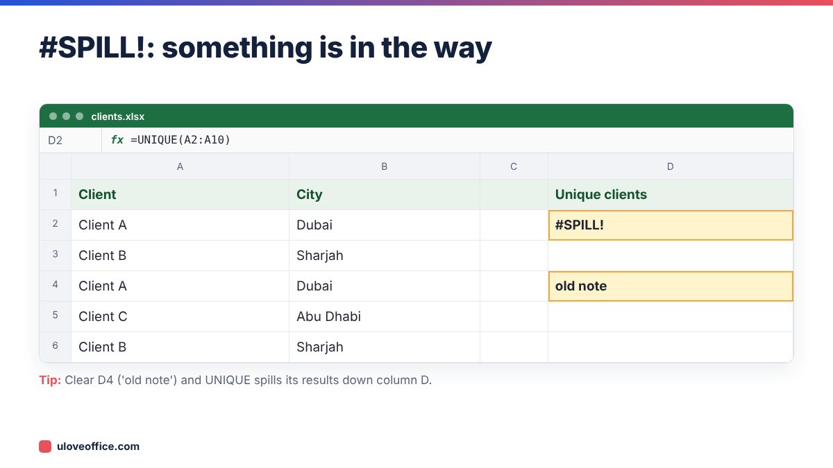
Dynamic array functions in Microsoft 365, such as FILTER, UNIQUE, SORT, SEQUENCE and TEXTSPLIT, return several results that “spill” into neighbouring cells. #SPILL! appears when they cannot.
Causes and fixes:
- Cells in the spill range are not empty. Even a space or an invisible character blocks it. Click the error, choose Select Obstructing Cells, and clear them.
- Merged cells in the way. Unmerge them.
- The formula is inside an Excel Table. Tables do not support spilling. Move the formula outside the table, or convert the table to a normal range.
- The result is too big for the sheet, for example referencing a whole column like
A:Ain some formulas. Limit the range, for exampleA2:A5000.
#N/A
#N/A means “not available” and usually comes from lookups: VLOOKUP, XLOOKUP, MATCH, INDEX/MATCH.
Causes and fixes:
- The value really is not in the list. Check spelling. Sometimes #N/A is the correct answer: the item is missing from your master list.
- Extra spaces. “Client A ” with a trailing space does not match “Client A”. Clean with
TRIMor Power Query. - Numbers stored as text. An invoice number
1045stored as text does not match the number1045. Convert with Data > Text to Columns orVALUE(), or match usingTEXT(). - Wrong lookup range. In VLOOKUP, the lookup value must be in the first column of the range. XLOOKUP avoids this problem. See our XLOOKUP vs VLOOKUP guide.
- Approximate match by mistake. VLOOKUP’s last argument should be
FALSE(or 0) for exact matches.
Showing a friendly result: once you know #N/A means “not found”, you can display something clearer:
=XLOOKUP(A2, Clients[ID], Clients[Name], "Not found")=IFNA(VLOOKUP(A2, Clients, 2, FALSE), "Not found")
Use IFNA rather than IFERROR here, so other errors still show.
#VALUE!
#VALUE! means a formula got the wrong kind of input.
Causes and fixes:
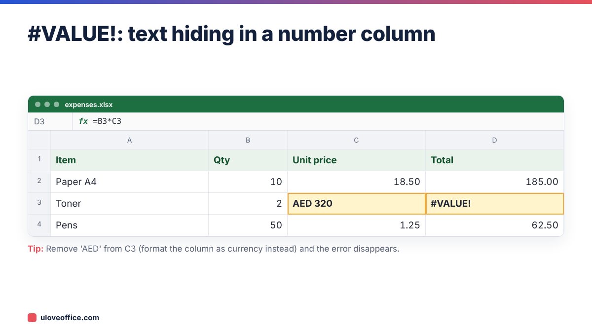
- Text in a calculation.
=A2+B2where B2 contains “AED 500” or “n/a”. Remove text from number cells, or useSUM(A2,B2), which ignores text. - Text dates. Date imported from a system as text. Convert to real dates; our Excel date formulas guide explains how.
- Hidden spaces or non-breaking spaces copied from web pages or PDFs. Use
=TRIM(SUBSTITUTE(A2,CHAR(160)," ")). - Ranges where single values are expected, in older Excel versions.
#REF!
#REF! means a formula points to a cell that no longer exists.
Causes and fixes:
- Deleted rows, columns or sheets that formulas referred to. Press Ctrl+Z immediately if you just did it. Otherwise, edit the formula to point to the right cells.
- Copying formulas that use relative references beyond the edge of the sheet.
- VLOOKUP column index too large, for example column 6 in a 5-column range.
- Broken links to other workbooks that were moved or deleted. Check Data > Edit Links.
Prevent it: use Excel Tables and structured references (Sales[Amount]), which adjust automatically, and avoid deleting columns that other sheets use. Lock important formula cells; see our guide on how to lock cells and protect formulas.
#DIV/0!
Division by zero or by an empty cell, common in percentage and average calculations.
Fixes:
- Check whether the divisor should really be zero.
- Show a blank or dash instead:
=IF(B2=0, "", A2/B2)or=IFERROR(A2/B2, ""). - For averages of empty ranges, use
AVERAGEIFor check the count first.
Our guide on calculating percentages in Excel has more examples.

#NAME?
Excel does not recognise something in the formula.
Causes and fixes:
- Misspelled function:
=VLOKUP(...). Use Excel’s autocomplete to avoid typos. - Text without quotes:
=IF(A2=Paid, ...)should be=IF(A2="Paid", ...). - Named range that does not exist or was deleted. Check Formulas > Name Manager.
- Function not available in your Excel version, for example
XLOOKUP,FILTERorTEXTSPLITin older versions. The file works for a colleague with Microsoft 365 but not for you.
#NUM!
Causes: impossible maths (square root of a negative number), an iterative function that cannot find a result (such as IRR with unusual cash flows), or a number too large for Excel. Check inputs and, for financial functions, try providing a guess value.
Hiding errors: when and how
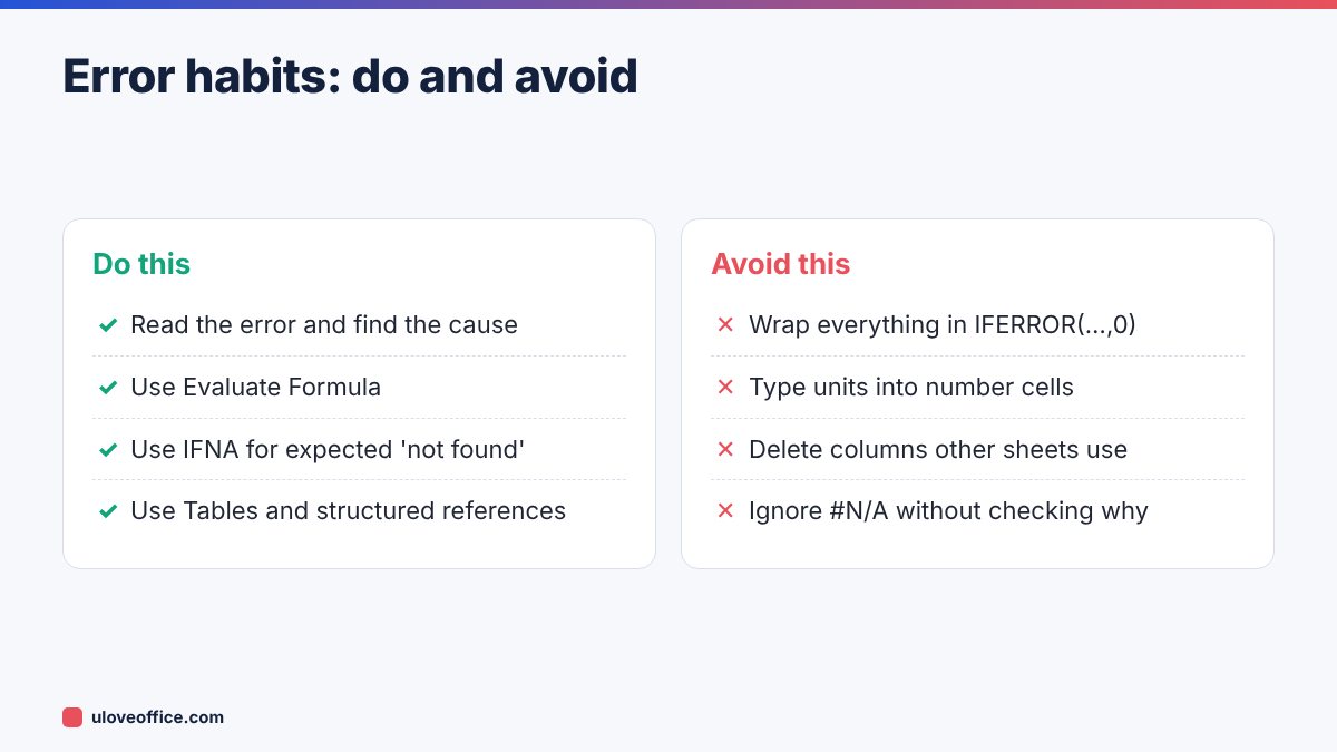
IFERROR is useful in finished reports, but use it carefully. Wrapping every formula in IFERROR(…, 0) hides real problems: a #REF! from a deleted column becomes a zero, and your total is quietly wrong.
Better practice:
- Fix the cause first.
- Use
IFNAfor lookups where “not found” is expected. - Use
IFERRORonly on the final presentation layer, with a visible message such as “Check” rather than zero.
Worked example: fixing a broken monthly report
An accountant opens the monthly sales report and sees errors everywhere. Working through them in order:
- #REF! in the summary sheet: someone deleted a “Region” column from the data sheet. Undo was no longer possible, so the formulas were updated to the correct column.
- #N/A in the client lookup: three new clients were not yet in the client master list. Added them.
- #VALUE! in totals: the new month’s export had prices with “AED” in the cell. Removed with Find and Replace.
- #SPILL! in the unique client list: an old note was sitting in the output column. Deleted.
Fifteen minutes later the report was correct, and the accountant converted the data range into an Excel Table to prevent the #REF! problem next month.
Preventing errors before they happen
Most errors come from the same few habits. A few settings and rules prevent them:
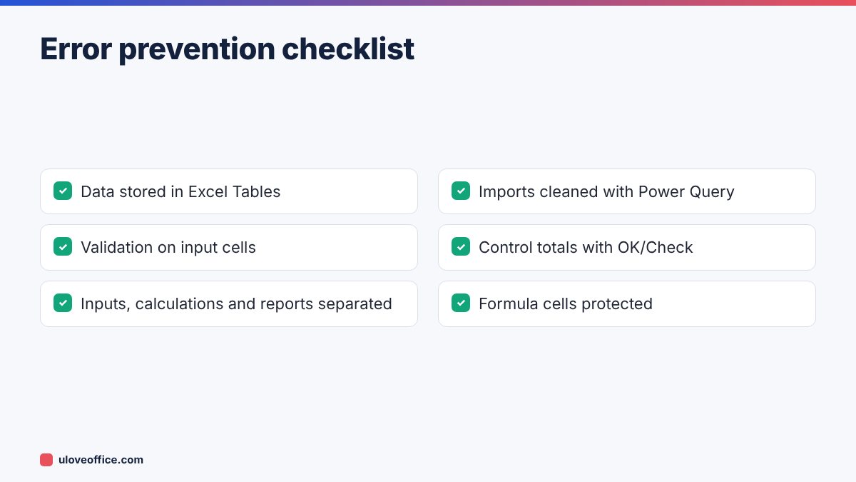
- Use Excel Tables (Ctrl+T) for data. Formulas use column names, adjust when rows are added and do not break when columns are reordered.
- Use data validation on input cells: numbers only, dates within a range, or a drop-down list. Our guide on creating a drop-down list in Excel shows how.
- Separate inputs, calculations and reports onto different sheets, and protect the calculation sheets.
- Clean imports with Power Query, which removes extra spaces, converts text numbers and fixes dates every time you refresh.
- Check totals with a control cell: a formula that compares two independent totals and shows “OK” or “Check”. If someone breaks something, the control cell tells you.
When you inherit a workbook full of errors, fix them in dependency order: start with the data sheet, then calculation sheets, then reports. Errors flow downstream, so fixing the source often clears dozens of report errors at once.
Key takeaways
- Each error type points to a specific cause; read it before fixing.
-
SPILL! is about the output range, #N/A about missing matches, #VALUE! about data types, #REF! about deleted references.
- Evaluate Formula and Trace Precedents find the problem cell quickly.
- Clean data (spaces, text numbers, text dates) prevents most errors.
- Hide errors only after you understand them, and never by turning them into zeros silently.
📘 Continue reading
Frequently asked questions
Why does my formula work on my colleague’s computer but show #NAME?
They probably have a newer Excel version with functions your version lacks.
How do I find all errors in a sheet?
Home > Find & Select > Go To Special > Formulas > Errors selects every error cell.
Can errors break a whole workbook?
Errors flow into every formula that depends on them. Fix the first error in the chain and the rest often disappear.
What does a green triangle mean?
It is a warning, not an error, such as a number stored as text or a formula that differs from its neighbours. Check it anyway.
Conclusion
Excel errors are clues. #SPILL! means clear the way, #N/A means check the match, #VALUE! means fix the data type, #REF! means repair the reference, #DIV/0! means handle zero. Use Evaluate Formula to find the cause, fix the data or formula, and hide errors only when you know why they appear. Your reports will be more accurate and much less stressful to maintain. If a file itself will not open, see our guide on how to repair a corrupted Excel file.
Last checked: 9 November 2026.