
Excel formulas for office work: 10 essentials for 2026
Excel formulas for office work: 10 essentials for 2026
Learn 10 Excel formulas for office work with practical examples for budgets, invoices, attendance and admin tasks. Includes formulas and an AED example.
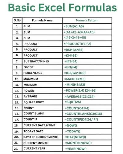
The most useful Excel formulas for office work in 2026 are SUM, AVERAGE, IF, COUNTIF, COUNTIFS, SUMIF, SUMIFS, XLOOKUP, IFERROR and TODAY. Together, they cover everyday jobs such as totaling expenses, checking budgets, counting attendance, summarizing invoices, finding employee or supplier details, handling formula errors and tracking deadlines. Excel formulas begin with an equals sign, and you can reuse a working formula across rows or recurring workbooks instead of calculating the same task manually. This guide shows what each formula does, how an office manager can use it, and the exact formula pattern to try.
How to use Excel formulas for office work
Start with a clean table: put one type of information in each column, use clear headers, and keep dates and amounts consistent. Select the cell where you want the result, type =, enter the function and its arguments, then press Enter. Microsoft confirms that Excel formulas start with an equals sign. Test the first result against a value you can verify manually before copying the formula down a large worksheet.
1. SUM: total expenses, invoices or petty cash
SUM adds values. For an office expense list with amounts in D2:D20, use =SUM(D2:D20). This is faster and safer than typing a long chain such as =D2+D3+D4. Office managers can use SUM for monthly stationery costs, travel claims, supplier invoices, event spending and departmental totals. When new data is added outside the selected range, remember to extend the range or use an Excel Table so your reporting structure stays easier to maintain.
2. AVERAGE: find a typical cost or response time
AVERAGE returns the arithmetic mean of numeric values. If delivery times in hours are stored in E2:E15, use =AVERAGE(E2:E15). This can help compare average courier time, average monthly utility cost, average meeting-room usage or average processing time. An average can hide unusually high or low values, so review the source rows when the result will influence a purchasing or staffing decision.
3. IF: turn a rule into an automatic result
IF returns one result when a condition is true and another when it is false. For a budget status, use =IF(D2>C2,”Over budget”,”Within budget”), where C2 is the approved amount and D2 is actual spending. The same pattern can flag overdue tasks, missing documents, low stock or completed approvals. Keep the test easy to understand so another employee can audit the workbook later.
4. COUNTIF: count one condition
COUNTIF counts cells that meet one criterion. Microsoft gives its basic structure as COUNTIF(range, criteria). If column F contains task status, =COUNTIF(F2:F100,”Pending”) counts pending tasks. You can also count a department name, a location, a specific attendance code or values above a threshold. It is particularly useful for quick dashboard figures when you need a count rather than a total amount.
5. COUNTIFS: count records that meet several conditions
COUNTIFS extends counting to multiple criteria. For example, =COUNTIFS(B2:B100,”Dubai”,F2:F100,”Pending”) counts records where the location is Dubai and the status is Pending. Microsoft states that COUNTIFS applies criteria across multiple ranges and counts cases where all criteria are met. Use it for tasks such as counting unpaid invoices for one supplier group or attendance records for a particular office and month.
6. SUMIF: total amounts matching one condition
SUMIF adds values that meet one criterion. If column B contains departments and column D contains expenses, =SUMIF(B2:B100,”Administration”,D2:D100) totals Administration expenses. This is useful for one-category reports such as spending by department, invoices from one vendor or purchases with one status. Microsoft documents SUMIF as the function for summing values based on criteria you specify.
7. SUMIFS: total amounts using multiple conditions
SUMIFS is one of the strongest Excel formulas for office work because it totals values only when several conditions are satisfied. Its structure begins with the sum range, followed by criteria ranges and criteria. For example, =SUMIFS(D2:D100,B2:B100,”Administration”,F2:F100,”Approved”) totals approved Administration expenses. Microsoft recommends SUMIFS when values need to be summed using multiple conditions.
8. XLOOKUP: find employee, supplier or asset details
XLOOKUP searches a range and returns the corresponding item from another range. For an employee ID in H2, =XLOOKUP(H2,A2:A100,B2:B100,”Not found”) can return the employee name from column B. Microsoft describes XLOOKUP as an improved lookup that can search in any direction and returns exact matches by default. It is ideal for employee directories, supplier lists, asset registers and price tables. Check compatibility if colleagues use older Excel versions.
9. IFERROR: replace confusing formula errors
IFERROR lets you display a cleaner result when another formula returns an error. A common office pattern is =IFERROR(XLOOKUP(H2,A2:A100,B2:B100),”Check ID”). Instead of leaving an error code in a report, the sheet tells the user what to do next. Do not use IFERROR to hide genuine data problems without investigation; first confirm why the underlying lookup or calculation can fail.
10. TODAY: keep deadline checks current
TODAY returns the current date and is useful in deadline formulas. If a due date is in G2, =IF(G2<TODAY(),”Overdue”,”Open”) can flag dates that have passed. Office managers can use TODAY for contract renewals, insurance reminders, document expiry, maintenance schedules and action trackers. Because the current date changes, a workbook using TODAY can update its result when Excel recalculates.
Worked example with AED figures
Assume an office manager has an approved monthly supplies budget of AED 12,000. The expense table contains AED 2,450 for stationery, AED 3,200 for printing, AED 1,850 for pantry supplies and AED 2,100 for courier services. With those four amounts in D2:D5, =SUM(D2:D5) returns AED 9,600. If the approved budget is in C1, =IF(SUM(D2:D5)>C1,”Over budget”,”Within budget”) returns “Within budget.” The remaining budget is AED 2,400, calculated with =C1-SUM(D2:D5).
Now assume column B labels each expense by category. The manager can use SUMIF or SUMIFS to create category totals without manually selecting individual rows. If a later AED 3,000 approved purchase is added, the total becomes AED 12,600 and the IF result changes to “Over budget.” This small example shows why formulas are useful: the worksheet responds to changed data instead of forcing the manager to rebuild every calculation.
How to use these formulas step by step
First, decide the business question: total, average, count, conditional result or lookup. Second, identify the cells that contain the source data. Third, choose the simplest formula that answers the question. Fourth, enter the formula in one result cell and verify it manually. Fifth, copy or fill it only after the first result is correct. Finally, document unusual assumptions in a nearby note or instructions sheet so the workbook remains understandable when another person takes over.
Can you use Excel formulas free unlimited times?
Excel does not charge per SUM, IF or XLOOKUP calculation. Once you have access to a version of Excel that supports a function, formulas can be reused throughout your workbook rather than purchased one calculation at a time. However, Excel itself may require an eligible Microsoft 365 subscription or software license, and function availability differs by version. Microsoft notes, for example, that XLOOKUP is not available as a native function in Excel 2016 or Excel 2019. So “free unlimited Excel formulas” should not be confused with free unlimited access to every Excel product or feature.
Frequently asked questions
What are the most useful Excel formulas for office work?
For general administration, start with SUM, AVERAGE, IF, COUNTIF, COUNTIFS, SUMIF, SUMIFS, XLOOKUP, IFERROR and TODAY. They cover common totals, conditions, counts, lookups and deadline checks without requiring advanced spreadsheet programming.
Which Excel formula should a beginner learn first?
Learn SUM first, then IF and COUNTIF. After those feel comfortable, move to SUMIFS and XLOOKUP. This sequence covers many everyday office tasks while gradually introducing criteria and lookup logic.
Is XLOOKUP better than VLOOKUP?
For supported Excel versions, Microsoft recommends trying XLOOKUP as an improved alternative. It can work in any direction and uses exact matching by default. VLOOKUP remains important when maintaining older workbooks or working with environments where XLOOKUP is unavailable.
What is the difference between SUMIF and SUMIFS?
SUMIF is designed for a single criterion, while SUMIFS supports multiple criteria. Use SUMIF for “total Administration expenses” and SUMIFS for “total approved Administration expenses in a particular reporting set.”
Where can I practice Excel formulas for office work?
Create a small sample workbook with fictional expenses, employees, tasks and due dates. Practice each formula on 10 to 20 rows and check the result manually. You can also use the Excel-related tools and guides on uloveoffice.com as part of your office-document workflow.
Conclusion
The best Excel formulas for office work are the ones that remove repetitive manual steps while keeping the workbook easy to check. Start with SUM, AVERAGE and IF, then add COUNTIF, COUNTIFS, SUMIF, SUMIFS, XLOOKUP, IFERROR and TODAY as your worksheets become more detailed. Save a tested example of each formula so you can reuse it in future budgets, trackers and reports. For more practical office-document tools and guides, visit uloveoffice.com.
Screenshots needed
- Step 1 – Example office worksheet with clean headers for department, status, amount and due date.
- Step 2 – SUM formula entered in the formula bar with the source range highlighted.
- Step 3 – IF formula showing a budget status result.
- Step 4 – SUMIFS example using department and approval status criteria.
- Step 5 – XLOOKUP example returning an employee or supplier name from an ID.
- Step 6 – TODAY-based deadline check showing Open and Overdue results.
- Step 7 – Final office dashboard or summary with calculated AED totals.
Internal links to add
- Target page: the most relevant Excel/spreadsheet tool or Excel formulas guide on uloveoffice.com – insert the exact live URL in the CMS.
- Related article: How to convert Excel to PDF – link to the matching live page if published.
- Related article: How to edit Excel files online – link to the matching live page if published.
- Related article: Office productivity or spreadsheet tips – link to the matching live article if published.
Sources for factual claims
- Microsoft Support – Overview of formulas in Excel: https://support.microsoft.com/en-us/Excel/get-started/overview-of-formulas-in-excel
- Microsoft Support – Excel functions by category: https://support.microsoft.com/en-us/office/excel-functions-by-category-5f91f4e9-7b42-46d2-9bd1-63f26a86c0eb
- Microsoft Support – XLOOKUP function: https://support.microsoft.com/en-us/excel/get-started/xlookup-function
- Microsoft Support – SUMIFS function: https://support.microsoft.com/en-us/excel/functions/sumifs-function
- Microsoft Support – COUNTIFS function: https://support.microsoft.com/en-us/excel/functions/countifs-function
Editorial note: Confirm the exact uloveoffice.com tool/article URLs before publication. Do not describe Excel itself as free unlimited software; formulas can be reused, but product licensing and function availability depend on the Excel version.